
Introduction
The llm routing cost latency quality formula is the missing piece between the advice and the actual decision. Everyone says to use llm routing so easy requests hit the cheap model, but almost nobody says how to score the trade between cost, latency, and quality, or how to check later whether the routing policy actually saved money without quietly hurting output.
This page is for the person building or tuning a model routing layer, whether that sits in app code, a gateway, or an n8n-style workflow. You’ll leave with a scoring function, a worked example, and the per-request telemetry to track, so routing becomes something you can measure and improve, not just a cost-saving slogan.
The Routing Formula in One Look
The formula is simple: a routing score is a weighted sum of normalized cost, normalized latency, and a quality proxy, each scaled from 0 to 1. In compact form:
Score = w_cost*C + w_latency*L + w_quality*Q, and you pick the highest scorer among the models that already clear your minimum quality floor.
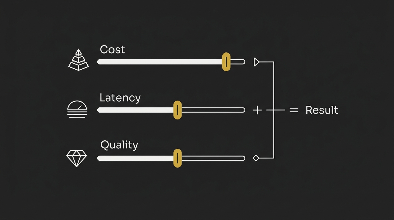
That structure matters because the best route is rarely the most capable model. It’s usually the model that gives enough quality for that request at the lowest acceptable cost and latency.
For the full guide, see our AI token costs calculator.
The scoring function
A routing score is one number per candidate model, computed from the same request and the same weights. Higher is better, but only after you exclude models that fail a hard quality threshold for the task.
In practice, that means two layers. First, filter out models that aren’t good enough for the job. Then score the remaining models with the weighted formula so the router can choose the cheapest fast-enough option, instead of defaulting to the strongest model every time.
What each term means
w_cost, w_latency, w_quality: the weights for cost, latency, and quality. They should add up to 1 so the routing score stays interpretable across requests.
C: the normalized cost term for that model on that request, scaled to 0 to 1 across the candidate set. Lower raw cost should map to a higher normalized score, otherwise the formula rewards expensive models by accident.
L: the normalized latency term, also scaled to 0 to 1 across the candidate set. Lower latency should map to a higher score, for the same reason.
Q: the normalized quality term or quality proxy, scaled to 0 to 1 across the candidate set. Higher measured or predicted quality should map to a higher score.
The useful rule is this: normalize all three terms onto the same 0 to 1 scale first, then apply weights. If you skip that step, raw milliseconds, dollars per million tokens, and quality metrics won’t be comparable, and the routing score stops meaning anything.
The Three-Way Trade, Stated Concretely
Routing to a cheaper model usually buys you lower inference cost and often lower latency, but the price gap is bigger than most teams assume. The same workload can swing by 100x or more in list price across cheap versus frontier models, so sending everything to the best model is often just overpaying. And the thing that catches people is output: input is rarely the budget killer, because output tokens are the expensive side on every major provider and often cost 3 to 5 times more than input.
So a model that looks cheap on paper can still become the most expensive option end to end if it produces long answers. Claude Opus 5 is priced at $5.00 per million input tokens and $25.00 per million output tokens, GPT-5.6 Sol at $5.00 input and $30.00 output, and Gemini 3.7 Flash at $0.75 input and $3.75 output.
What you gain moving to a cheaper model
Moving a narrow class of requests to a cheaper model cuts cost fast when the task is simple and the answer is short. Classification, extraction, and tight summaries are the usual wins, because the model has less room to generate costly extra output and the route decision is easier to defend.
You also tend to get a speed gain, especially when the cheaper model is smaller and the completion is shorter. But that saving only holds if the routed slice is actually simple enough, otherwise you save cents on list price and lose dollars in retries, fallbacks, or rework.
What you risk losing
What you risk losing is response quality, and the failure is usually silent. The dangerous version is not an obvious crash. It’s the answer that looks fine, misses one key detail, makes a weak tool call, or drifts just enough that nobody notices until support tickets or manual review catch it later.
Why does this bite so often? Because dashboards show cost and latency immediately, but they don’t show a quiet drop in answer quality unless you built for it. A route that looks cheaper can be more expensive in practice when the model needs second passes, human cleanup, or escalation after the first answer failed.
Picking the Weights and Working One Example
You set the weights by starting with what failure looks like in the app, not by splitting importance evenly. If a chat surface lives or dies on responsiveness, latency gets the heavier weight. If the work runs overnight in batches, cost should carry more of the score. And if the task is high-stakes, like a legal summary, quality is not just another weighted term, it should be a hard gate before any route is allowed to compete.

A simple way to make the decision consistent is to turn product priorities into rules:
- For an interactive chat request, weight latency highest, then quality, then cost.
- For a batch classification or enrichment task, weight cost highest, then quality, then latency.
- For a high-risk task, set a minimum quality threshold first, then score only the models that clear it.
Why do this first? Because the same scoring formula can produce the wrong route if low-quality candidates are allowed into a high-risk pool, or if a cheap model wins a user-facing request just because nobody priced the UX hit properly.
Normalize cost
Estimate input and output tokens for the request class, multiply by each model’s live per-token rates, then scale those costs from 0 to 1 across the candidate set.
Normalize latency
Use your own measured latency for this request path, not guessed numbers. Record the same latency metric for each candidate model, then scale it from fastest to slowest.
Set the quality proxy
Choose one measurable pass signal for the task, like label accuracy, tool-call success, or schema-valid output rate, and score each model on the same test set.
Apply weights
Multiply each normalized term by its weight. A support triage flow might favor cost, while a user-facing assistant might put more weight on latency.
Pick the winner
Choose the model with the best final score among the candidates that clear any hard quality floor. Then monitor if that route still wins once real traffic shifts.
How to set the weights from what the app cares about
A latency-critical app should weight latency high because user perception starts before the full answer finishes. For a live chat request, a practical starting point is to make latency the largest term, then let quality break ties, then let cost matter only after the first two are acceptable.
A batch job should weight cost high because the user never feels the difference between 900 ms and 1.8 seconds if the output lands later in a queue. In that task, the better decision is often the cheaper route that still clears the quality bar, especially when the rate spread between candidate models is already large.
A high-stakes workflow should set a hard quality floor before scoring anything else. If a legal-summary request needs citation fidelity or a strict pass rate on an eval set, any model below that floor is out, even if it is faster or cheaper.
A worked example with live per-token rates
Take a short support classification request checked against live standard API pricing from the provider rate cards dated 2026-08-21. Assume one request uses 800 input tokens and 120 output tokens, and the candidate route set is GPT-5.6 Sol, Claude Opus 5, Gemini 3.7 Flash, and DeepSeek-V4-Flash.
Using the published rates per 1M tokens, the estimated per-request API cost is:
| Model | Input rate | Output rate | Estimated request cost |
|---|---|---|---|
| GPT-5.6 Sol | $5.00 | $30.00 | $0.0076 |
| Claude Opus 5 | $5.00 | $25.00 | $0.0070 |
| Gemini 3.7 Flash | $0.75 | $3.75 | $0.0011 |
| DeepSeek-V4-Flash (off-peak) | $0.22 | $0.66 | $0.0003 |
That spread is the point. On a small classification task, the route can differ by more than 20x in direct model cost before you even factor in cache hits or off-peak scheduling.
Now run the score. First, normalize cost across these four options from cheapest to most expensive. Second, plug in the latency numbers you actually measure for this request path. Third, add a quality proxy from a labeled test set, for example exact-label accuracy on 200 past support tickets.
If this is a batch support task, a sensible starting weight set is cost 0.6, quality 0.3, latency 0.1. If Gemini 3.7 Flash and DeepSeek-V4-Flash are both above your minimum classification accuracy, the cheaper one will usually win the decision unless measured latency or error rate shifts the score back the other way.
If this is a live support widget, change the weights before you change the model. The same request might move to latency 0.5, quality 0.3, cost 0.2, and the winning route can flip once real TTFT and completion times are included. Cost calculators are useful here, but the route decision is only honest when token price and measured latency sit in the same score.
For estimating those token totals before rollout, the simplest next step is a token estimator tied to real prompts and expected outputs. One high-conviction routing rule beats ten pretty dashboards.
Estimating the Cost Term Before You Have Data
You can estimate the cost term before launch with a simple per-request formula: expected input tokens plus expected output tokens, each multiplied by that model’s live rates for the request class you expect to send. Do this per model, per task type, because classification, RAG, and chat don’t produce the same output volume, and output tokens can move inference cost more than most teams expect.
A practical starting point is to bucket your traffic into 2 to 4 task classes, assign an expected input size to each, then apply an output ratio instead of guessing raw completions from scratch. A 20% output ratio is a solid default for many retrieval and chat tasks, so a 2,000-token prompt starts with roughly 400 output tokens; classification usually lands lower, while long-form tasks land much higher. That gives you a clean first-pass cost estimate without waiting for production logs.
Don’t stop at fresh input pricing, because cached input is usually the biggest discount on the entire rate card and ignoring it will overstate cost. On current published pricing, cache reads can be about 10x cheaper than fresh input on models like Claude Opus 5, GPT-5.6 Sol, and Gemini 3.7 Flash, and about 31x cheaper on DeepSeek-V4-Flash. For the full math, live rates, and output presets, estimate your AI token costs instantly.
Quality Proxies You Can Compute Without a Human Grader
You can score the Q term without a human grader by using computable proxies that track whether a model gives the right kind of output for the task. They are proxies, not truth, but they are good enough to route on if you keep them task-specific and treat them as gates rather than a replacement for judgment.
The useful mindset is simple: measure quality at the point where failure becomes visible. For extraction, that may be schema validity. For classification, it may be pass rate against a labeled set. For a cheap-first router, it may be how often the cheap model clears the bar without escalation.
Cheap-versus-expensive agreement on a sample
Agreement on a labeled sample is a practical proxy when you want to know whether the cheap model is close enough to the stronger one for a specific task. Run both models on the same benchmark, compare outputs against the expected answer, and track where the cheaper model matches acceptable results often enough to trust it on that route.
This works because routing is local, not global. You do not need a universal model ranking. You need to know whether Model A is good enough for support-tag classification, field extraction, or short summarization, and that usually shows up fast on a task-specific sample.
A simple way to use it:
- Build a small labeled sample for one task class.
- Run the cheap and expensive model on the same inputs.
- Check each output against the expected answer or label.
- Record agreement rate and failure types, not just averages.
The weakness is obvious: agreement can hide shared mistakes. If both models miss the same edge case, the number looks clean while the quality is still weak. And if you mix task classes in one sample, the signal gets blurry fast.
Task pass rates and escalation rate
Task pass rates are often the cleanest proxy because they measure whether the output met the task’s minimum bar. For structured work, that can be schema validation. For generation with repeated trials, it can be self-consistency across multiple runs. For simple routed work, teams also watch whether the cheap model’s answer is accepted often enough to keep it on that lane.
Why is this usable for the Q term? Because it turns quality into a binary or rate-based signal the router can act on. A parsed JSON object, a valid SQL shape, or a stable repeated output is not the whole story, but it is a reliable first filter for whether the result is safe to keep.
Common pass-rate checks include:
- Schema validation for structured outputs
- Rule checks for required fields or formats
- Self-consistency across repeated generations
- Acceptance or pass behavior on clearly defined simple tasks
Escalation rate is the companion signal. In a cheap-first setup, it tells you how often the lower-cost model fails the gate and has to hand off to a stronger model. If that rate climbs, quality at the cheap tier is drifting, the verifier got stricter, or the task mix changed.
Its weakness is that escalation rate is indirect. A low escalation rate can mean the cheap model is doing well, or it can mean your gate is too loose. A high pass rate has the same problem. So use these signals together: pass rate tells you what clears, escalation rate tells you how often it fails, and the benchmark sample checks whether the gate still maps to real quality by task class.
For a plain-language foundation on tokens and how model inputs are counted, see what a token means in AI.
When Cheap-First Escalation Costs More Than Going Expensive
Cheap-first only saves money when the cheap model resolves enough requests. Once the escalation rate gets too high, you are paying for two attempts on too many requests, and the blended cost can end up above routing straight to the expensive model first.
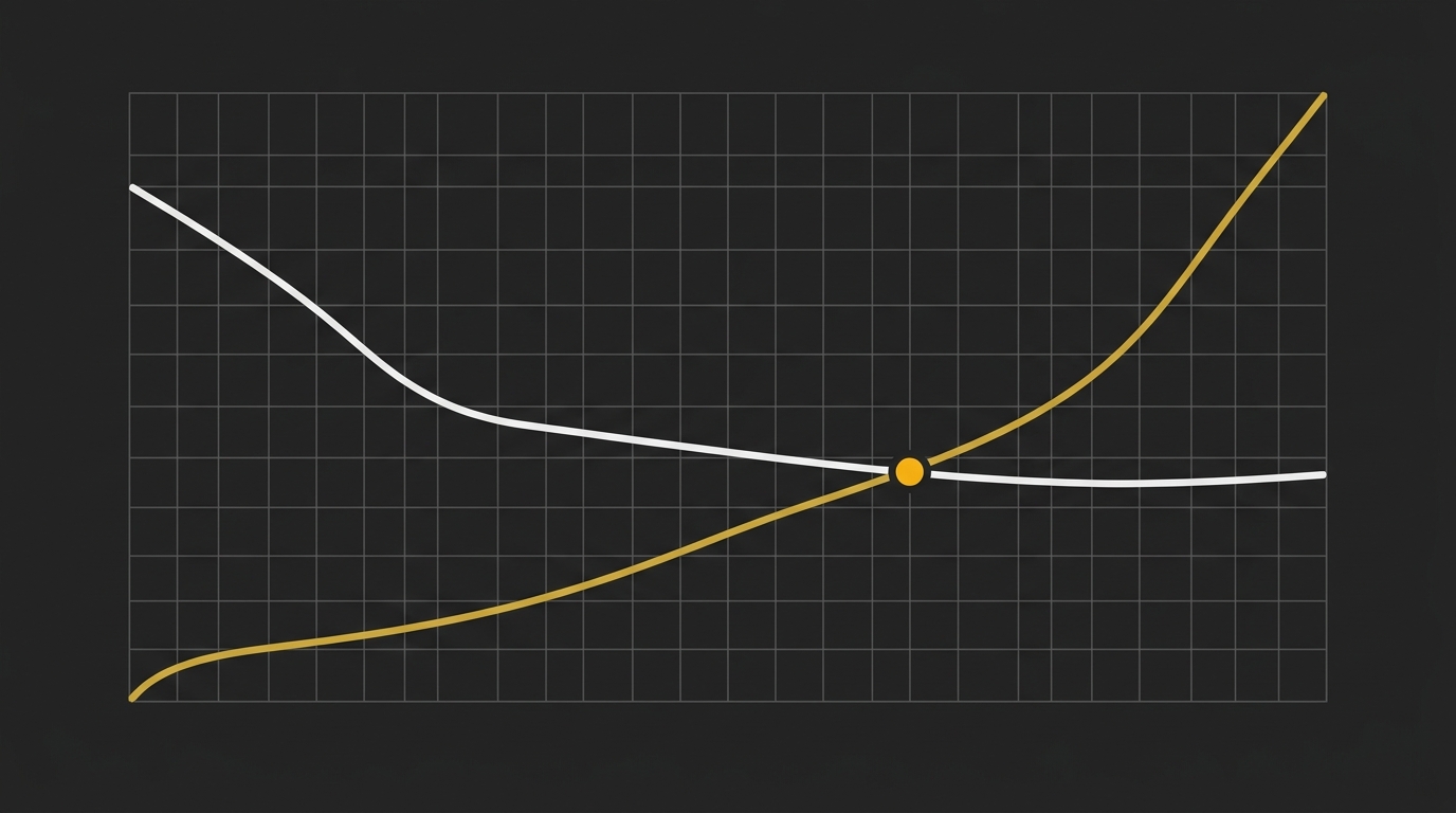
That is the trap with model cascades. They look efficient on paper, but the live variable is not the cheap model’s list price, it is the share of traffic that has to be retried. If that retry share drifts because your validator got stricter, your prompts changed, or a provider started formatting differently, the route’s economics flip fast.
| Approach | Cost per request | Expected cost at escalation rate e | When the lines cross |
|---|---|---|---|
| Expensive-first | One expensive call | E | Baseline |
| Cheap-then-escalate | One cheap call on every request, plus an expensive call on escalations | C + e × E | Crosses when C + e × E > E, so e > 1 – (C / E) |
| Example: cheap is 20% of expensive | C = 0.2E | 0.2E + e × E | Break-even at e = 80% |
| Example: cheap is 10% of expensive | C = 0.1E | 0.1E + e × E | Break-even at e = 90% |
The escalation pattern
Cheap-first gets worse when escalation stops being the exception and starts being normal traffic. If 30% of requests escalate, the extra cheap attempt is usually worth it. If 85% escalate, that same route is now paying the cheap toll almost every time before paying the full expensive bill anyway.
What counts as escalation is broader than a hard model failure. It can be schema validation misses, low-confidence outputs, a judge rejecting the answer, or a timeout that triggers fallback to another model. Different trigger, same bill.
There is a second failure mode people miss: retry logic can distort the math even when upstream models are healthy. If cooldown rules and replica retries bounce requests between workers, you can underuse available capacity while still stacking extra attempts, which pushes both latency and cost in the wrong direction.
The break-even arithmetic
The arithmetic is simple: expensive-first costs E per request, while a cheap-first route costs C + e × E, where C is the cheap attempt and e is the escalation rate. Cheap-first is cheaper only when C + e × E < E.
Rearrange that and you get the decision rule: cheap-first works only when e < 1 - (C / E). Say your cheap model costs one-fifth of the expensive one. The break-even escalation rate is 80%. Above that, going straight to the expensive model is cheaper.
That threshold is the useful part, because it gives you something to monitor per route instead of arguing in the abstract. A cascade with a 5x price gap can still be a bad system if verification is too strict or retries start ping-ponging across replicas. One high escalation rate can wipe out the headline savings.
What to Instrument Per Request
A routing policy is only as good as the per-request data behind it. If you don’t log the model choice, token usage, cache behavior, latency, escalation path, and computed cost for each request, the formula looks smart on paper but stays blind in production.
The one field most teams miss is cache hit rate. That’s the number that exposes silent prompt bugs that never throw an error, like a timestamp added to a system block, a tool list rebuilt on every call, or prompt text that mutates between turns, because the failure shows up as cost instead of a broken output.
| Field | What question it answers later | Why the policy is blind without it |
|---|---|---|
| Model used | Which model actually handled this request? | You can’t compare planned routing versus real routing, or spot fallback drift. |
| Input tokens | What did the request cost to send in? | You can’t price the prompt side of the decision or normalize model cost fairly. |
| Output tokens | What did the model cost to generate back? | You miss completion-heavy tasks where a cheap input rate still becomes expensive. |
| Cached tokens | How much of the request reused prior context? | You can’t tell whether savings came from routing, caching, or neither. |
| Latency | How long did this request take end to end? | You can’t tune the latency term or prove a cheaper route was actually faster. |
| Route decision | Why was this model selected? | You lose the reason code needed to debug rules, weights, intent classification, or thresholds. |
| Escalation flag | Did this request require a second pass on a stronger model? | You can’t measure cascade rate, which is one of the main cost variables. |
| Computed cost | What did this request actually cost under the route taken? | You end up with weekly totals instead of per-request economics, so savings stay unprovable. |
The fields to record
The minimum useful record is small: model used, input tokens, output tokens, cached tokens, latency, route decision, escalation flag, and computed cost. That gives you enough data to explain both the router’s choice and the bill that followed from that choice.
But don’t log them as disconnected counters. Store them on the same request trace or event so you can answer practical questions later: which requests escalated, whether the cheap tier was actually cheaper after retries, and whether cache savings were real or were wiped out by prompt churn.
A simple checklist looks like this:
- Model identifier actually called
- Input token count
- Output token count
- Cached token count
- End-to-end latency
- Route reason or policy branch
- Escalated: yes or no
- Computed per-request cost
Cache hit rate deserves its own derived metric, even though it comes from cached tokens over eligible tokens. Why? Because this is where silent bugs show up. A prompt can still produce correct answers while missing cache on every turn, and without that data the problem looks like normal spend.
Mapping them to standard tracing attributes
The clean way to map this into observability is to put stable facts on the trace span and roll the same fields into metrics. In practice, that means request-level attributes such as model name, route reason, token counts, cached token counts, escalation status, and computed cost, plus latency as the span duration or a paired metric.
If you’re using OpenTelemetry-style tracing, think in two layers. First, attributes on the LLM or gateway span describe what happened on this request. Second, metrics aggregate those same fields across the system in production, so you can chart cost by route, cache hit rate by agent, and escalation rate by model pair.
A practical mapping looks like this:
| Field | Trace attribute example | Metric you can derive |
|---|---|---|
| Model used | llm.model.name |
requests by model |
| Input tokens | llm.usage.input_tokens |
input tokens by route |
| Output tokens | llm.usage.output_tokens |
output tokens by model |
| Cached tokens | llm.usage.cached_tokens |
cache hit rate |
| Latency | span duration | p50/p95 latency by route |
| Route decision | routing.reason or routing.policy |
route distribution |
| Escalation flag | routing.escalated=true |
escalation rate |
| Computed cost | llm.cost.usd |
cost per request, route, or agent |
The key is consistency. Teams often have model logs in one place, token billing in another, and latency in a gateway dashboard, then wonder why routing savings are hard to prove. One request, one record, one cost story. That’s the setup that keeps the formula honest.
Keeping the Formula Honest Over Time
Keep the formula tied to the job the request is actually doing. In latency-critical apps, weight latency harder because a slower answer is the failure. In batch jobs, push harder on cost because a few extra seconds usually do not matter. For quality-sensitive work, set a hard floor first, then route among the models that clear it, because the cheapest bad answer is still a bad answer in production.

Re-check the inputs on a schedule, not just the weights. Model pricing moves, promotional rates expire, and a number that looked safe in Q3 can break your unit economics in Q1. One concrete example: Gemini 3.7 Flash and 3.6 Flash run at promotional rates through 31 December 2026, then on 1 January 2027 the rates double from $0.75 to $1.50 for input and from $3.75 to $7.50 for output. If your router still scores that model on the old rate card, the formula is lying to you.
Next steps are simple: keep the routing logic, but refresh the live price assumptions before they drift. If you need a plain-English reset on token units first, read What Is a Token in AI Large Language Models. Then Estimate your AI token costs instantly and re-price the cost term with current rates.
Frequently Asked Questions
How do you pick the weights in a routing formula?
You pick the weights by starting with the app’s failure condition, then weighting the term that most directly avoids that failure. If a user-facing chat flow breaks when answers feel slow, latency gets more weight. If the task is a batch workflow with predictable deadlines, cost can take more weight, while quality gets pushed hardest on tasks where a wrong answer is expensive.
The practical move is to avoid equal weights by default. Routing works better when the weights reflect what the request is actually trying to do, not a generic average across every workload.
Can you change routing weights and models without restarting the gateway?
Yes, that’s one of the main reasons teams put routing logic at the gateway layer. When the gateway already normalizes provider APIs, adding a model, removing one, or reweighting candidates can be handled as a policy or configuration change instead of a worker restart and code redeploy.
That matters operationally because teams often want to react to price changes, latency drift, or a new model release on the same day. The cleaner setup is: the gateway owns dynamic model selection, and the application still owns the task definition and eval criteria.
How much can model routing actually save?
Model routing can cut spend hard, and 60 to 90 percent savings is realistic when a large share of traffic can be resolved by cheaper models. The actual number depends on traffic mix, the price gap between tiers, and how often requests escalate.
Why the spread? Because savings come from distribution, not from the formula alone. If most of your requests are lightweight classification, extraction, or structured output jobs, routing can land close to the high end; if most traffic already needs frontier-level reasoning, savings compress fast.
When does cheap-first escalation cost more than going expensive first?
Cheap-first costs more when too many requests fail the first pass and escalate, because you’re then paying for two calls on a large share of traffic. Once the escalation rate gets high enough, the blended cost can overtake sending the request to the stronger model first.
That’s the break-even idea in plain terms: compare one expensive call against one cheap call plus the probability-weighted expensive fallback. In model cascades, the escalation rate is not a side metric, it’s the number that decides whether the route is saving money or quietly burning it.
How do you measure quality for routing without a human grader?
You measure quality with computable proxies that track whether the output meets the job’s requirements. Common examples are schema validation, pass rates on known test cases, agreement with a stronger model on a sample, or whether a first-pass answer escalates.
But keep the proxy stable. If you’re also relying on prompt caching, changing cached components mid-session, like the system prompt or rolling context window, can silently wipe out the expected cache benefit and distort the routing picture you think you’re measuring.
Should routing live in the gateway or the application?
Routing usually belongs in the gateway, because that’s where cross-model policy, provider normalization, and live cost and latency telemetry naturally sit. It lets teams change routes centrally instead of editing application code every time a model mix changes.
The application still owns one part that shouldn’t be pushed down: the definition of acceptable output. Put differently, the gateway decides where to send the request, but the app decides what good looks like.